enrichment function

%load_ext autoreload
%autoreload 2

import greatpy as great
import pandas as pd
from math import inf
from numpy import log,nan, int64,cov,corrcoef
from scipy.stats import pearsonr
from seaborn import scatterplot as sp
import matplotlib.pyplot as plt

import warnings
warnings.filterwarnings('ignore')

Compute the p-values

test = "../data/tests/test_data/input/03_srf_hg19.bed"
regdom = "../data/human/hg19/regulatory_domain.bed"
great_out = "../data/tests/test_data/output/03_srf_hg19_output_great_webserver.tsv"
size = "../data/human/hg19/chr_size.bed"

enrichment = great.tl.enrichment(
    test_file = test,
    regdom_file = regdom,
    chr_size_file = size,
    annotation_file = "../data/human/ontologies.csv",
    binom = True,
    hypergeom = True,
    )
enrichment = great.tl.set_fdr(enrichment)
enrichment = great.tl.set_bonferroni(enrichment)
enrichment

	go_term	binom_p_value	binom_fold_enrichment	hypergeom_p_value	hypergeometric_fold_enrichment	intersection_size	recall	binom_fdr	hypergeom_fdr	binom_bonferroni	hypergeom_bonferroni
GO:0072749	cellular response to cytochalasin B	2.21968e-12	2.27251e+05	4.28032e-02	2.33627e+01	5	5.00000e+00	4.61693e-09	4.65089e-01	9.23386e-09	1.00000e+00
GO:0051623	positive regulation of norepinephrine uptake	2.21968e-12	2.27251e+05	4.28032e-02	2.33627e+01	5	5.00000e+00	4.61693e-09	4.65089e-01	9.23386e-09	1.00000e+00
GO:0098973	structural constituent of postsynaptic actin c...	2.11740e-10	9.10526e+04	1.60543e-01	5.84068e+00	5	1.25000e+00	2.93613e-07	5.43858e-01	8.80839e-07	1.00000e+00
GO:0097433	dense body	6.40085e-10	1.60618e+04	1.41783e-03	1.16814e+01	8	1.33333e+00	6.65688e-07	3.65408e-01	2.66275e-06	1.00000e+00
GO:0032796	uropod organization	2.69880e-09	5.45449e+04	1.82991e-03	2.33627e+01	5	2.50000e+00	1.93909e-06	3.65408e-01	1.12270e-05	1.00000e+00
...	...	...	...	...	...	...	...	...	...	...	...
GO:0007156	homophilic cell adhesion via plasma membrane a...	9.99960e-01	1.12747e+02	9.84651e-01	3.89379e-01	3	1.66667e-02	1.00000e+00	1.00000e+00	1.00000e+00	1.00000e+00
GO:0007186	G protein-coupled receptor signaling pathway	9.99992e-01	2.46644e+02	1.00000e+00	3.07404e-01	19	1.47059e-02	1.00000e+00	1.00000e+00	1.00000e+00	1.00000e+00
GO:0016021	integral component of membrane	9.99997e-01	3.94493e+02	9.99998e-01	7.05221e-01	112	2.88958e-02	1.00000e+00	1.00000e+00	1.00000e+00	1.00000e+00
GO:0005887	integral component of plasma membrane	1.00000e+00	2.81852e+02	9.99970e-01	5.84068e-01	40	2.50000e-02	1.00000e+00	1.00000e+00	1.00000e+00	1.00000e+00
GO:0005886	plasma membrane	1.00000e+00	3.98798e+02	1.00000e+00	2.55733e-01	159	1.06776e-02	1.00000e+00	1.00000e+00	1.00000e+00	1.00000e+00

4160 rows × 11 columns

Compare p values between binomial and hypergeometric tests

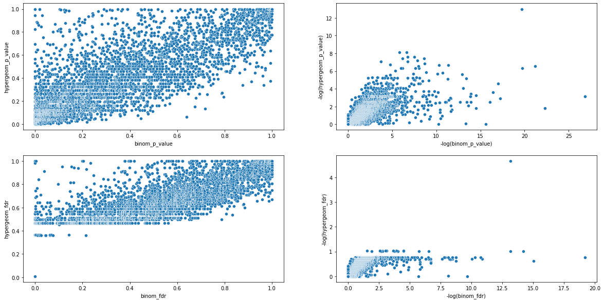
fig,ax = plt.subplots(2,2,figsize = (20,10))
great.pl.scatterplot(
    enrichment,
    "binom_p_value",
    "hypergeom_p_value",
    minus_log10 = False,ax = ax[0,0])
great.pl.scatterplot(
    enrichment,
    "binom_p_value",
    "hypergeom_p_value",
    minus_log10 = True,ax = ax[0,1])
great.pl.scatterplot(
    enrichment,
    "binom_fdr",
    "hypergeom_fdr",
    minus_log10 = False,ax = ax[1,0])
great.pl.scatterplot(
    enrichment,
    "binom_fdr",
    "hypergeom_fdr",
    minus_log10 = True,ax = ax[1,1])
plt.show()

pd.options.display.float_format = "{:.3f}".format
pd.DataFrame({
        "binom_vs_hyper": [cov(m = list(enrichment["binom_p_value"]), y = list(enrichment["hypergeom_p_value"]))[0][1],pearsonr(list(enrichment["binom_p_value"]), list(enrichment["hypergeom_p_value"]))[0]],
        "binom_fdr_vs_hyper_fdr":[cov(m = list(enrichment["binom_fdr"]), y = list(enrichment["hypergeom_fdr"]))[0][1],pearsonr(list(enrichment["binom_fdr"]), list(enrichment["hypergeom_fdr"]))[0]]},
        index = ["cov","pearson"])

	binom_vs_hyper	binom_fdr_vs_hyper_fdr
cov	0.062	0.030
pearson	0.773	0.758

The covariance between the binomial and hypergeometric values is very close to 0 (e-2). There is therefore no or little correlation between the variance of these two data

As we can see here, the correlation is quite good (~``0.75``) between the binomial and hypergeometric values returned by great.

We can explain this difference by the fact that the two statistical tests are not susceptible to the same biases and are therefore complementary.

The biases for the two tests are :

• The hypergeometric test may be biased by the size of the regulatory domains of the genes since isolated genes have very large regulatory domains and are therefore more likely to generate false positives

• The binomial test can also be biased if a large number of genomic regions to be tested are associated with a small set of genes that can also generate false positives